Dynamic Time Warping Algorithm Explained (Python)

In this world which is getting dominated by Internet of Things (IoT), there is an increasing need to understand signals from devices installed in households, shopping malls, factories and offices. For example, any voice assistant detects, authenticates and interprets commands from humans even if it is slow or fast. Our voice tone tends to be different during different times of the day. In the early morning after we get up from bed, we interact with a slower, heavier and lazier tone compared to other times of the day. These devices treat the signals as time series and compare the peaks, troughs and slopes by taking into account the varying lags and phases in the signals to come up with a similarity score. One of the most common algorithms used to accomplish this is Dynamic Time Warping (DTW). It is a very robust technique to compare two or more Time Series by ignoring any shifts and speed.

As part of Walmart Real Estate team, I am working on understanding the energy consumption pattern of different assets like refrigeration units, dehumidifiers, lighting, etc. installed in the retail stores.This will help in improving quality of data collected from IoT sensors, detect and prevent faults in the systems and improve energy consumption forecasting and planning. This analysis involves time series of energy consumption during different times of a day i.e. different days of a week, weeks of a month and months of a year. Time series forecasting often gives bad predictions when there is sudden shift in phase of the energy consumption due to unknown factors. For example if the defrost schedule, items refresh routine for a refrigeration unit, or weather changes suddenly and are not captured to explain the phase shifts of energy consumption, it is important to detect these change points.

In the example below, the items refresh routine of a store has shifted by 2 hours on Tuesday leading the shift in peak energy consumption of refrigeration units and this information was not available to us for many such stores.

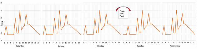
The peak at 2 am got shifted to 4 am. DTW when run recursively for consecutive days can identify the cases for which phase shift occurred without much change in shape of signals.

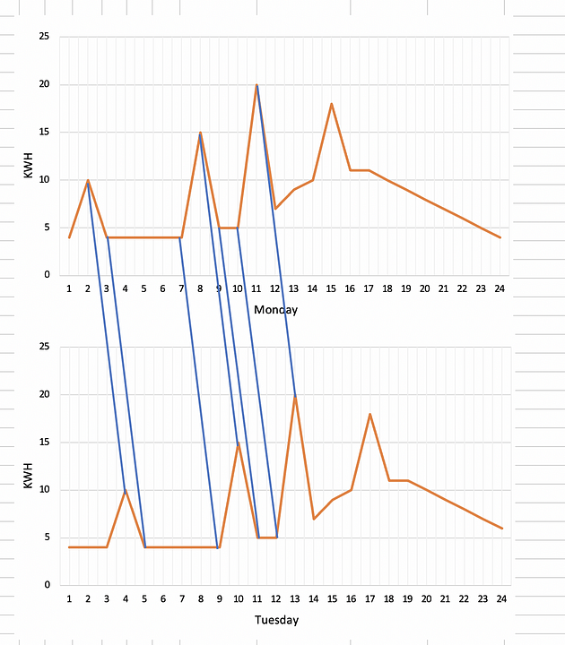
The training data can be restricted to Tuesday onwards to improve the prediction of energy consumption in future in this case as phase shift was detected on Tuesday. The setup improved the predictions substantially ( > 50%) for the stores for which the reason of shift was not known. This was not possible by traditional ways of one to one comparison of signals.

In this blog, I will explain how DTW algorithm works and throw some light on the calculation of the similarity score between two time series and its implementation in python. Most of the contents in this blog have been sourced from this paper, also mentioned in the references section below.

2. Why do we need DTW ?

Any two time series can be compared using euclidean distance or other similar distances on a one to one basis on time axis. The amplitude of first time series at time T will be compared with amplitude of second time series at time T. This will result into a very poor comparison and similarity score even if the two time series are very similar in shape but out of phase in time.

DTW compares amplitude of first signal at time T with amplitude of second signal at time T+1 and T-1 or T+2 and T-2. This makes sure it does not give low similarity score for signals with similar shape and different phase.

3. How it works?

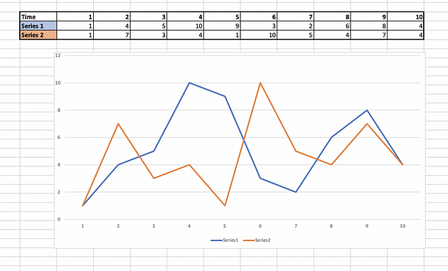
Let us take two time series signals P and Q

Series 1 (P) : 1,4,5,10,9,3,2,6,8,4

Series 2 (Q): 1,7,3,4,1,10,5,4,7,4

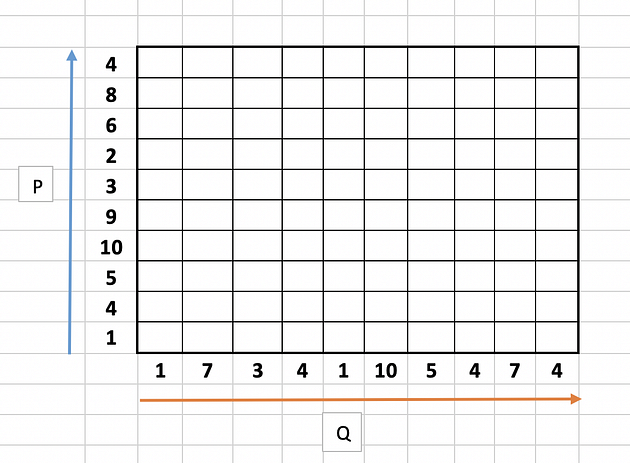
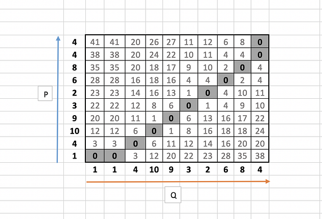
Step 1 : Empty Cost Matrix Creation

Create an empty cost matrix M with x and y labels as amplitudes of the two series to be compared.

Step 2: Cost Calculation

Fill the cost matrix using the formula mentioned below starting from left and bottom corner.

M(i, j) = |P(i) --- Q(j)| + min ( M(i-1,j-1), M(i, j-1), M(i-1,j) )

where

M is the matrix

i is the iterator for series P

j is the iterator for series Q

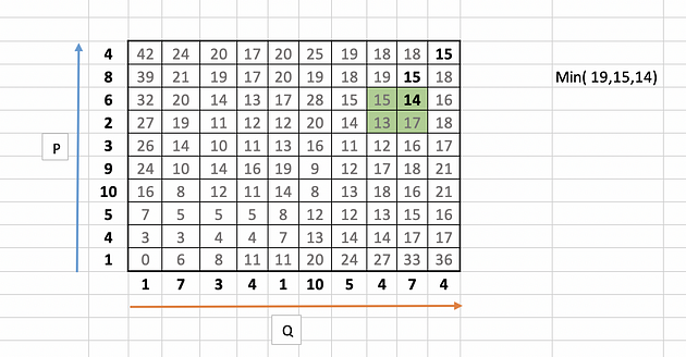
Let us take few examples (11,3 and 8 ) to illustrate the calculation as highlighted in the below table.

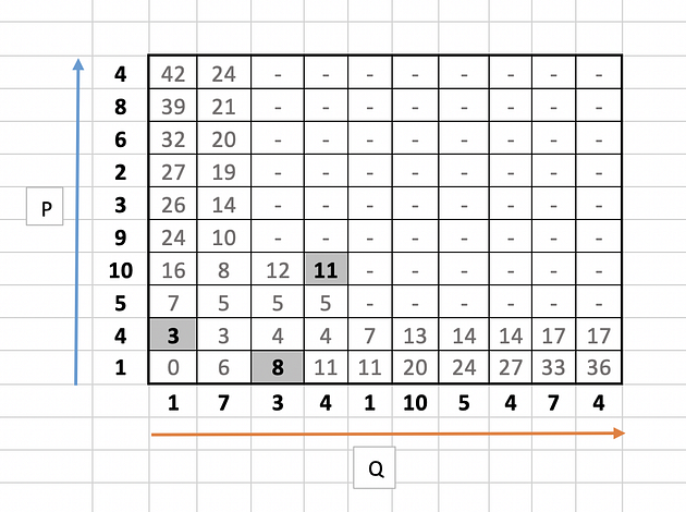
for 11,

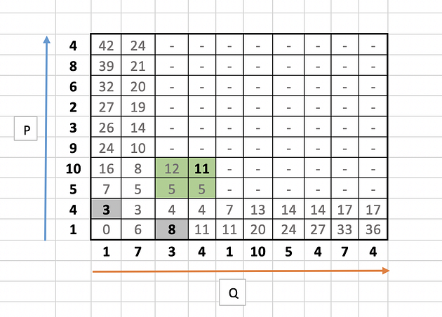
|10 --4| + min( 5, 12, 5 )

= 6 + 5

= 11

Similarly for 3,

|4 --1| + min( 0 )

= 3+ 0

= 3

and for 8,

|1 --3| + min( 6)

= 2 + 6

= 8

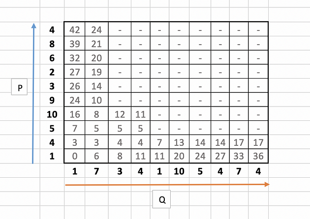
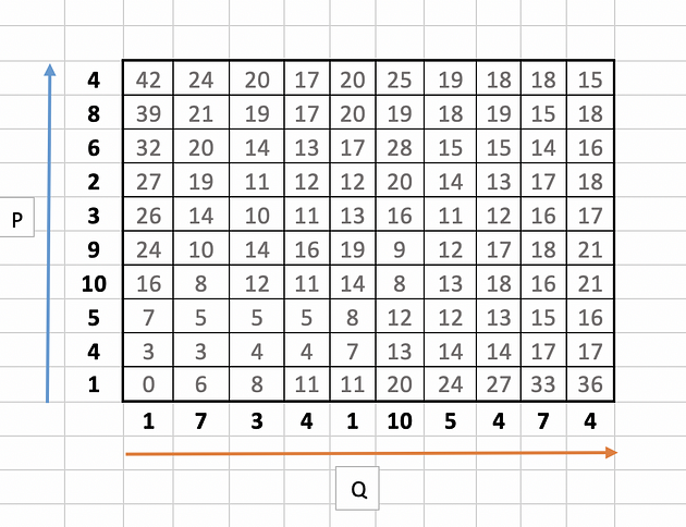
The full table will look like this:

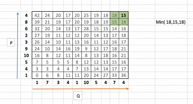
Step 3: Warping Path Identification

Identify the warping path starting from top right corner of the matrix and traversing to bottom left. The traversal path is identified based on the neighbour with minimum value.

In our example it starts with 15 and looks for minimum value i.e. 15 among its neighbours 18, 15 and 18.

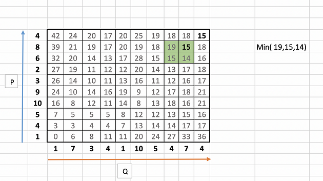
The next number in the warping traversal path is 14. This process continues till we reach the bottom or the left axis of the table.

The final path will look like this:

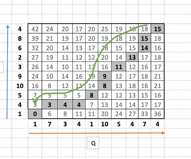
Let this warping path series be called as d.

d = [15,15,14,13,11,9,8,8,4,4,3,0]

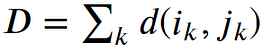
Step 4: Final Distance Calculation

Time normalised distance , D

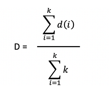
where k is the length of the series d.

k = 12 in our case.

D = ( 15 + 15 + 14 + 13 + 11 + 9 + 8 + 8 + 4 + 4 + 3 + 0 ) /12

= 104/12

= 8.63

Let us take another example with two very similar time series with unit time shift difference.

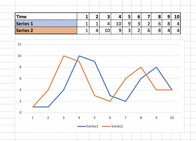
Cost matrix and warping path will look like this.

DTW distance ,D =

( 0 + 0 + 0 + 0 + 0 +0 +0 +0 +0 +0 +0 ) /11

= 0

Zero DTW distance implies that the time series are very similar and that is indeed the case as observed in the plot.

Resummation (Spaced Repitition)

Dynamic Time Warping (DTW) is a way to compare two -usually temporal- sequences that do not sync up perfectly. It is a method to calculate the optimal matching between two sequences. DTW is useful in many domains such as speech recognition, data mining, financial markets, etc. It's commonly used in data mining to measure the distance between two time-series.

In this post, we will go over the mathematics behind DTW. Then, two illustrative examples are provided to better understand the concept. If you are not interested in the math behind it, please jump to examples.

Formulation

Let's assume we have two sequences like the following:

𝑋=𝑥[1], 𝑥[2], ..., x[i], ..., x[n]

Y=y[1], y[2], ..., y[j], ..., y[m]

The sequences 𝑋 and 𝑌 can be arranged to form an 𝑛-by-𝑚 grid, where each point (𝑖, j) is the alignment between 𝑥[𝑖] and 𝑦[𝑗].

A warping path 𝑊 maps the elements of 𝑋 and 𝑌 to minimize the distance between them. 𝑊 is a sequence of grid points (𝑖, 𝑗). We will see an example of the warping path later.

Warping Path and DTW distance

The Optimal path to (𝑖𝑘, 𝑗𝑘) can be computed by:

where 𝑑 is the Euclidean distance. Then, the overall path cost can be calculated as

Restrictions on the Warping function

The warping path is found using a dynamic programming approach to align two sequences. Going through all possible paths is "combinatorically explosive" [1]. Therefore, for efficiency purposes, it's important to limit the number of possible warping paths, and hence the following constraints are outlined:

• Boundary Condition: This constraint ensures that the warping path begins with the start points of both signals and terminates with their endpoints.

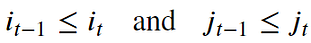
• Monotonicity condition: This constraint preserves the time-order of points (not going back in time).

• Continuity (step size) condition: This constraint limits the path transitions to adjacent points in time (not jumping in time).

In addition to the above three constraints, there are other less frequent conditions for an allowable warping path:

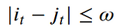
• Warping window condition: Allowable points can be restricted to fall within a given warping window of width 𝜔 (a positive integer).

• Slope condition: The warping path can be constrained by restricting the slope, and consequently avoiding extreme movements in one direction.

An acceptable warping path has combinations of chess king moves that are:

• Horizontal moves: (𝑖, 𝑗) → (𝑖, 𝑗+1)
• Vertical moves: (𝑖, 𝑗) → (𝑖+1, 𝑗)
• Diagonal moves: (𝑖, 𝑗) → (𝑖+1, 𝑗+1)

Implementation

Let's import all python packages we need.

import pandas as pd
import numpy as np# Plotting Packages
import matplotlib.pyplot as plt
import seaborn as sbn# Configuring Matplotlib
import matplotlib as mpl
mpl.rcParams['figure.dpi'] = 300
savefigoptions = dict(format="png", dpi=300, bboxinches="tight")# Computation packages
from scipy.spatial.distance import euclidean
from fastdtw import fastdtw

Let's define a method to compute the accumulated cost matrix D for the warp path. The cost matrix uses the Euclidean distance to calculate the distance between every two points. The methods to compute the Euclidean distance matrix and accumulated cost matrix are defined below:

Example 1

In this example, we have two sequences x and y with different lengths.

Create two sequences\

x = [3, 1, 2, 2, 1]
y = [2, 0, 0, 3, 3, 1, 0]

We cannot calculate the Euclidean distance between x and y since they don't have equal lengths.

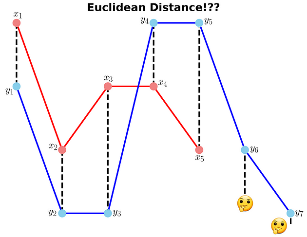
Example 1: Euclidean distance between x and y (is it possible? 🤔) (Image by Author)

Compute DTW distance and warp path

Many Python packages calculate the DTW by just providing the sequences and the type of distance (usually Euclidean). Here, we use a popular Python implementation of DTW that is FastDTW which is an approximate DTW algorithm with lower time and memory complexities [2].

dtwdistance, warppath = fastdtw(x, y, dist=euclidean)

Note that we are using SciPy's distance function Euclidean that we imported earlier. For a better understanding of the warp path, let's first compute the accumulated cost matrix and then visualize the path on a grid. The following code will plot a heatmap of the accumulated cost matrix.

costmatrix = computeaccumulatedcostmatrix(x, y)

Example 1: Python code to plot (and save) the heatmap of the accumulated cost matrix

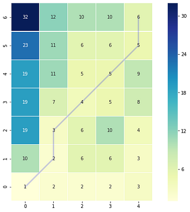
Example 1: Accumulated cost matrix and warping path (Image by Author)

The color bar shows the cost of each point in the grid. As can be seen, the warp path (blue line) is going through the lowest cost on the grid. Let's see the DTW distance and the warping path by printing these two variables.

DTW distance: 6.0
Warp path: [(0, 0), (1, 1), (1, 2), (2, 3), (3, 4), (4, 5), (4, 6)]

The warping path starts at point (0, 0) and ends at (4, 6) by 6 moves. Let's also calculate the accumulated cost most using the functions we defined earlier and compare the values with the heatmap.

costmatrix = computeaccumulatedcostmatrix(x, y)
print(np.flipud(cost_matrix)) # Flipping the cost matrix for easier comparison with heatmap values!>>> [[32. 12. 10. 10. 6.]
[23. 11. 6. 6. 5.]
[19. 11. 5. 5. 9.]
[19. 7. 4. 5. 8.]
[19. 3. 6. 10. 4.]
[10. 2. 6. 6. 3.]
[ 1. 2. 2. 2. 3.]]

The cost matrix is printed above has similar values to the heatmap.

Now let's plot the two sequences and connect the mapping points. The code to plot the DTW distance between x and y is given below.

Example 1: Python code to plot (and save) the DTW distance between x and y

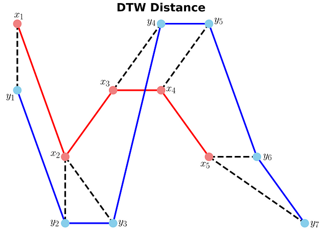
Example 1: DTW distance between x and y (Image by Author)

Example 2

In this example, we will use two sinusoidal signals and see how they will be matched by calculating the DTW distance between them.

Example 2: Generate two sinusoidal signals (x1 and x2) with different lengths

Just like Example 1, let's calculate the DTW distance and the warp path for *x1 *and *x2 *signals using FastDTW package.

distance, warp_path = fastdtw(x1, x2, dist=euclidean)

Example 2: Python code to plot (and save) the DTW distance between x1 and x2

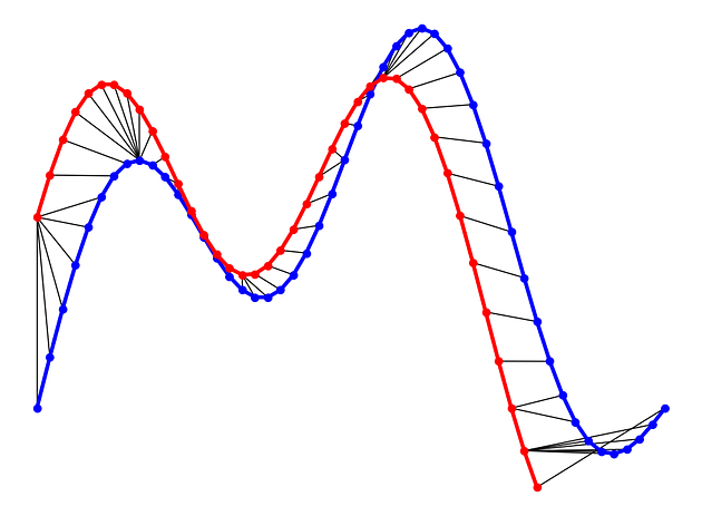
Example 2: DTW distance between x1 and x2 (Image by Author)

As can be seen in above figure, the DTW distance between the two signals is particularly powerful when the signals have similar patterns. The extrema (maximum and minimum points) between the two signals are correctly mapped. Moreover, unlike Euclidean distance, we may see many-to-one mapping when DTW distance is used, particularly if the two signals have different lengths.

You may spot an issue with dynamic time warping from the figure above. Can you guess what it is?

The issue is around the head and tail of time-series that do not properly match. This is because the DTW algorithm cannot afford the warping invariance for at the endpoints. In short, the effect of this is that a small difference at the sequence endpoints will tend to contribute disproportionately to the estimated similarity[3].

Conclusion

DTW is an algorithm to find an optimal alignment between two sequences and a useful distance metric to have in our toolbox. This technique is useful when we are working with two non-linear sequences, particularly if one sequence is a non-linear stretched/shrunk version of the other. The warping path is a combination of "chess king" moves that starts from the head of two sequences and ends with their tails.

You can find the Jupyter notebook for this blog post here. Thanks for reading!

References

[1] Donald J. Berndt and James Clifford, Using Dynamic Time Warping to Find Patterns in Time Series, 3rd International Conference on Knowledge Discovery and Data Mining

[2] Salvador, S. and P. Chan, FastDTW: Toward accurate dynamic time warping in linear time and space(2007), Intelligent Data Analysis

[3] Diego Furtado Silva, et al., On the effect of endpoints on dynamic time warping (2016), SIGKDD Workshop on Mining and Learning from Time Series

Useful Links

[1] https://nipunbatra.github.io/blog/ml/2014/05/01/dtw.html

[2] https://databricks.com/blog/2019/04/30/understanding-dynamic-time-warping.html

Sounds like time traveling or some kind of future technic, however, it is not. Dynamic Time Warping is used to compare the similarity or calculate the distance between two arrays or time series with different length.

Suppose we want to calculate the distance of two equal-length arrays:

a = [1, 2, 3]
b = [3, 2, 2]

How to do that? One obvious way is to match up a and b in 1-to-1 fashion and sum up the total distance of each component. This sounds easy, but what if a and b have different lengths?

a = [1, 2, 3]
b = [2, 2, 2, 3, 4]

How to match them up? Which should map to which? To solve the problem, there comes dynamic time warping. Just as its name indicates, to warp the series so that they can match up.

Use Cases

Before digging into the algorithm, you might have the question that is it useful? Do we really need to compare the distance between two unequal-length time series?

Yes, in a lot of scenarios DTW is playing a key role.

Sound Pattern Recognition

One use case is to detect the sound pattern of the same kind. Suppose we want to recognise the voice of a person by analysing his sound track, and we are able to collect his sound track of saying Hello in one scenario. However, people speak in the same word in different ways, what if he speaks hello in a much slower pace like Heeeeeeelloooooo , we will need an algorithm to match up the sound track of different lengths and be able to identify they come from the same person.

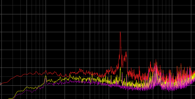
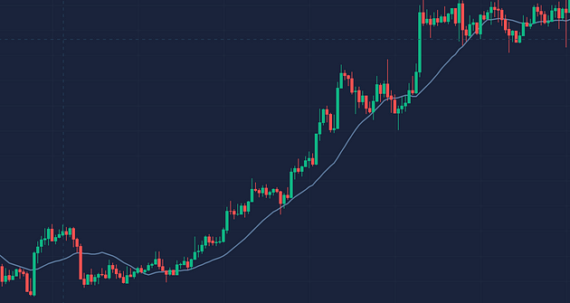
Stock Market

In a stock market, people always hope to be able to predict the future, however using general machine learning algorithms can be exhaustive, as most prediction task requires test and training set to have the same dimension of features. However, if you ever speculate in the stock market, you will know that even the same pattern of a stock can have very different length reflection on klines and indicators.

Definition & Idea

A concise explanation of DTW from wiki,

In time series analysis, dynamic time warping (DTW) is one of the algorithms for measuring similarity between two temporal sequences, which may vary in speed. DTW has been applied to temporal sequences of video, audio, and graphics data --- indeed, any data that can be turned into a linear sequence can be analysed with DTW.

The idea to compare arrays with different length is to build one-to-many and many-to-one matches so that the total distance can be minimised between the two.

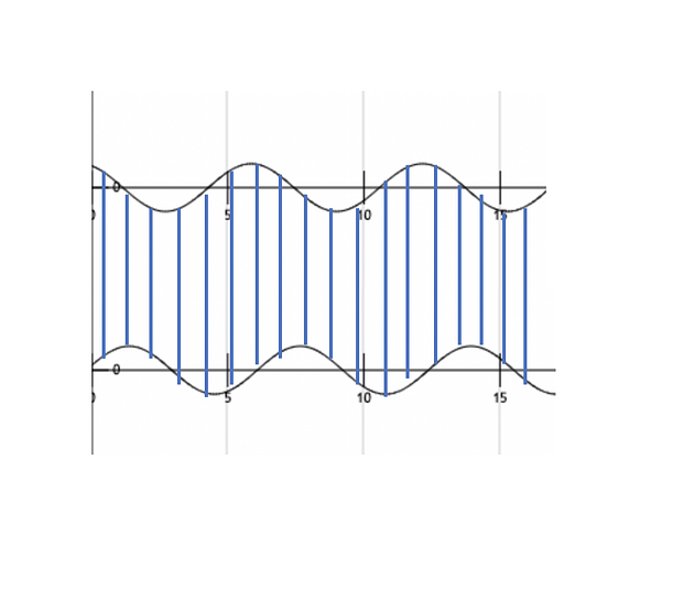
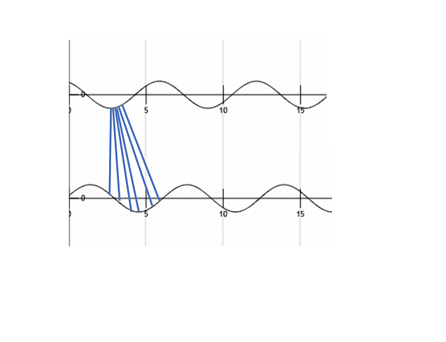
Suppose we have two different arrays red and blue with different length:

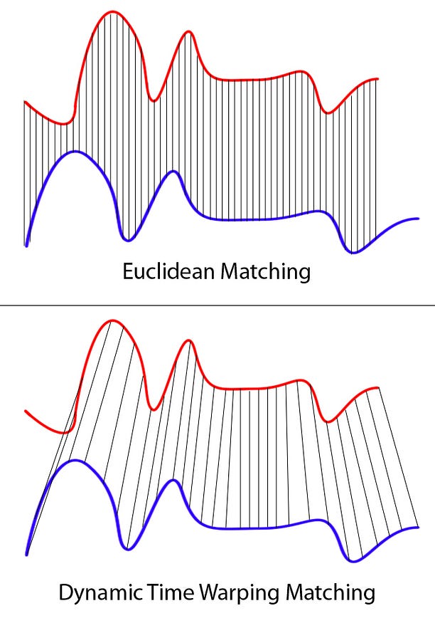
Clearly these two series follow the same pattern, but the blue curve is longer than the red. If we apply the one-to-one match, shown in the top, the mapping is not perfectly synced up and the tail of the blue curve is being left out.

DTW overcomes the issue by developing a one-to-many match so that the troughs and peaks with the same pattern are perfectly matched, and there is no left out for both curves(shown in the bottom top).

Rules

In general, DTW is a method that calculates an optimal match between two given sequences (e.g. time series) with certain restriction and rules(comes from wiki):

• Every index from the first sequence must be matched with one or more indices from the other sequence and vice versa
• The first index from the first sequence must be matched with the first index from the other sequence (but it does not have to be its only match)
• The last index from the first sequence must be matched with the last index from the other sequence (but it does not have to be its only match)
• The mapping of the indices from the first sequence to indices from the other sequence must be monotonically increasing, and vice versa, i.e. if j > i are indices from the first sequence, then there must not be two indices l > k in the other sequence, such that index i is matched with index l and index j is matched with index k , and vice versa

The optimal match is denoted by the match that satisfies all the restrictions and the rules and that has the minimal cost, where the cost is computed as the sum of absolute differences, for each matched pair of indices, between their values.

To summarise is that head and tail must be positionally matched, no cross-match and no left out.

Implementation

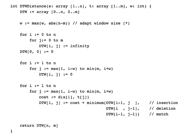
The implementation of the algorithm looks extremely concise:

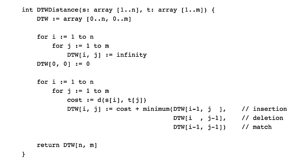
where DTW[i, j] is the distance between s[1:i] and t[1:j] with the best alignment.

The key lies in:

DTW[i, j] := cost + minimum(DTW[i-1, j ],
DTW[i , j-1],
DTW[i-1, j-1])

Which is saying that the cost of between two arrays with length i and j equals the distance between the tails + the minimum of cost in arrays with length _*i-1, j* , *i, j-1* , and *i-1, j-1* ._

Put it in python would be:

Example:

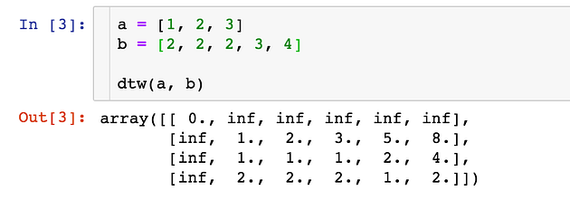
The distance between a and b would be the last element of the matrix, which is 2.

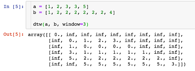
Add Window Constraint

One issue of the above algorithm is that we allow one element in an array to match an unlimited number of elements in the other array(as long as the tail can match in the end), this would cause the mapping to bent over a lot, for example, the following array:

a = [1, 2, 3]
b = [1, 2, 2, 2, 2, 2, 2, 2, ..., 5]

To minimise the distance, the element 2 in array a would match all the 2 in array b , which causes an array b to bent severely. To avoid this, we can add a window constraint to limit the number of elements one can match:

The key difference is that now each element is confined to match elements in range i --- w and i + w . The w := max(w, abs(n-m)) guarantees all indices can be matched up.

The implementation and example would be:

Apply a Package

There is also contributed packages available on Pypi to use directly. Here I demonstrate an example using fastdtw:

It gives you the distance of two lists and index mapping(the example can extend to a multi-dimension array).