
Overview
REST is a generally agreed-upon set of principles and constraints. They are recommendations, not a standard.
// inside /api/apiRoutes.js <- this can be place anywhere and called anything
const express = require('express');

// if the other routers are not nested inside /api then the paths would change
const userRoutes = require('./users/userRoutes');
const productRoutes = require('./products/productRoutes');
const clientRoutes = require('./clients/clientRoutes');

const router = express.Router(); // notice the Uppercase R

// this file will only be used when the route begins with "/api"
// so we can remove that from the URLs, so "/api/users" becomes simply "/users"
router.use('/users', userRoutes);
router.use('/products', productRoutes);
router.use('/clients', clientRoutes);

// .. and any other endpoint related to the user's resource

// after the route has been fully configured, we then export it so it can be required where needed
module.exports = router; // standard convention dictates that this is the last line on the file
Overview
Foreign keys are a type of table field used for creating links between tables. Like primary keys, they are most often integers that identify (rather than store) data. However, whereas a primary key is used to id rows in a table, foreign keys are used to connect a record in one table to a record in a second table.
Follow Along
Consider the following farms and ranchers tables.
The farm_id in the ranchers table is an example of a foreign key. Each entry in the farm_id (foreign key) column corresponds to an id (primary key) in the farms table. This allows us to track which farm each rancher belongs to while keeping the tables normalized.
If we could only see the ranchers table, we would know that John, Jane, and Jen all work together and that Jim and Jay also work together. However, to know where any of them work, we would need to look at the farms table.
Challenge
Open SQLTryIT (Links to an external site.).
How many records in the products table belong to the category "confections"?
Objective 2 — query data from multiple tables
Now that we understand the basics of querying data from a single table, let's move on to selecting data from multiple tables using JOIN operations.
Overview
We can use a JOIN to combine query data from multiple tables using a single SELECT statement.
There are different types of joins; some are listed below:
- inner joins.
- outer joins.
- left joins.
- right joins.
- cross joins.
- non-equality joins.
- self joins.
Using joins requires that the two tables of interest contain at least one field with shared information. For example, if a departments table has an id field, and an employee table has a departmentid_ field, and the values that exist in the id column of the departments table live in the departmentid_ field of the employee table, we can use those fields to join both tables like so:
select * from employees
join departments on employees.department_id = departments.id
This query will return the data from both tables for every instance where the ON condition is true. If there are employees with no value for departmentid or where the value stored in the field does not correspond to an existing id in the departments table, then that record will NOT be returned. In a similar fashion, any records from the departments table that don't have an employee associated with them will also be omitted from the results. Basically, if the id* does not show as the value of department_id for an employee, it won't be able to join.
We can shorten the condition by giving the table names an alias. This is a common practice. Below is the same example using aliases, picking which fields to return and sorting the results:
select d.id, d.name, e.id, e.first_name, e.last_name, e.salary
from employees as e
join departments as d
  on e.department_id = d.id
order by d.name, e.last_name
Notice that we can take advantage of white space and indentation to make queries more readable.
There are several ways of writing joins, but the one shown here should work on all database management systems and avoid some pitfalls, so we recommend it.
The syntax for performing a similar join using Knex is as follows:
db('employees as e')
  .join('departments as d', 'e.department_id', 'd.id')
  .select('d.id', 'd.name', 'e.first_name', 'e.last_name', 'e.salary')
Follow Along
A good explanation of how the different types of joins can be seen in this article from w3resource.com (Links to an external site.).
Challenge
Use this online tool (Links to an external site.) to write the following queries:
- list the products, including their category name.
- list the products, including the supplier name.
- list the products, including both the category name and supplier name.
What is SQL Joins?
An SQL JOIN clause combines rows from two or more tables. It creates a set of rows in a temporary table.
How to Join two tables in SQL?
A JOIN works on two or more tables if they have at least one common field and have a relationship between them.
JOIN keeps the base tables (structure and data) unchanged.
Join vs. Subquery
- JOINs are faster than a subquery and it is very rare that the opposite.
- In JOINs the RDBMS calculates an execution plan, that can predict, what data should be loaded and how much it will take to processed and as a result this process save some times, unlike the subquery there is no pre-process calculation and run all the queries and load all their data to do the processing.
- A JOIN is checked conditions first and then put it into table and displays; where as a subquery take separate temp table internally and checking condition.
- When joins are using, there should be connection between two or more than two tables and each table has a relation with other while subquery means query inside another query, has no need to relation, it works on columns and conditions.
SQL JOINS: EQUI JOIN and NON EQUI JOIN
The are two types of SQL JOINS — EQUI JOIN and NON EQUI JOIN
- SQL EQUI JOIN :
The SQL EQUI JOIN is a simple SQL join uses the equal sign(=) as the comparison operator for the condition. It has two types — SQL Outer join and SQL Inner join.
- SQL NON EQUI JOIN :
The SQL NON EQUI JOIN is a join uses comparison operator other than the equal sign like >, <, >=, <= with the condition.
SQL EQUI JOIN : INNER JOIN and OUTER JOIN
The SQL EQUI JOIN can be classified into two types — INNER JOIN and OUTER JOIN
- SQL INNER JOIN
This type of EQUI JOIN returns all rows from tables where the key record of one table is equal to the key records of another table.
- SQL OUTER JOIN
This type of EQUI JOIN returns all rows from one table and only those rows from the secondary table where the joined condition is satisfying i.e. the columns are equal in both tables.
In order to perform a JOIN query, the required information we need are:
a) The name of the tablesb) Name of the columns of two or more tables, based on which a condition will perform.
Syntax:
FROM table1
join_type table2
[ON (join_condition)]
Parameters:
Pictorial Presentation of SQL Joins:
Sample table: company
Sample table: foods
To join two tables 'company' and 'foods', the following SQL statement can be used :
SQL Code:
SELECT  company.company_id,company.company_name,
foods.item_id,foods.item_name
FROM company,foods;
Copy
Output:
COMPAN COMPANY_NAME              ITEM_ID  ITEM_NAME
------ ------------------------- -------- ---------------
18     Order All                 1        Chex Mix
18     Order All                 6        Cheez-It
18     Order All                 2        BN Biscuit
18     Order All                 3        Mighty Munch
18     Order All                 4        Pot Rice
18     Order All                 5        Jaffa Cakes
18     Order All                 7        Salt n Shake
15     Jack Hill Ltd             1        Chex Mix
15     Jack Hill Ltd             6        Cheez-It
15     Jack Hill Ltd             2        BN Biscuit
15     Jack Hill Ltd             3        Mighty Munch
15     Jack Hill Ltd             4        Pot Rice
15     Jack Hill Ltd             5        Jaffa Cakes
15     Jack Hill Ltd             7        Salt n Shake
16     Akas Foods                1        Chex Mix
16     Akas Foods                6        Cheez-It
16     Akas Foods                2        BN Biscuit
16     Akas Foods                3        Mighty Munch
16     Akas Foods                4        Pot Rice
16     Akas Foods                5        Jaffa Cakes
16     Akas Foods                7        Salt n Shake
.........
.........
.........
JOINS: Relational Databases
Key points to remember:
Click on the following to get the slides presentation -
Practice SQL Exercises
- SQL Exercises, Practice, Solution
- SQL Retrieve data from tables [33 Exercises]
- SQL Boolean and Relational operators [12 Exercises]
- SQL Wildcard and Special operators [22 Exercises]
- SQL Aggregate Functions [25 Exercises]
- SQL Formatting query output [10 Exercises]
- SQL Quering on Multiple Tables [7 Exercises]
- FILTERING and SORTING on HR Database [38 Exercises]
- SQL JOINS
- SQL JOINS [29 Exercises]
- SQL JOINS on HR Database [27 Exercises]
- SQL SUBQUERIES
- SQL SUBQUERIES [39 Exercises]
- SQL Union[9 Exercises]
- SQL User Account Management [16 Exercise]
- Movie Database
- BASIC queries on movie Database [10 Exercises]
- Soccer Database
- Introduction
- JOINS
- Hospital Database
- Introduction
- BASIC, SUBQUERIES, and JOINS [39 Exercises]
- Employee Database
- BASIC queries on employee Database [115 Exercises]
- SUBQUERIES on employee Database [77 Exercises]
- More to come!
Objective 3 — write database access methods
Overview
While we can write database code directly into our endpoints, best practices dictate that all database logic exists in separate, modular methods. These files containing database access helpers are often called models
Follow Along
To handle CRUD operations for a single resource, we would want to create a model (or database access file) containing the following methods:
function find() {
}

function findById(id) {
}

function add(user) {
}

function update(changes, id) {
}

function remove(id) {
}
Each of these functions would use Knex logic to perform the necessary database operation.
function find() {
  return db('users');
}
For each method, we can choose what value to return. For example, we may prefer findById() to return a single user object rather than an array.
function findById(id) {
// first() returns the first entry in the db matching the query
  return db('users').where({ id }).first();
}
We can also use existing methods like findById() to help add() return the new user (instead of just the id).
function add(user) {
  db('users').insert(user)
    .then(ids => {
      return findById(ids[0]);
    });
}
Once all methods are written as desired, we can export them like so:
module.exports = {
  find,
  findById,
  add,
  update,
  delete,
}
…and use the helpers in our endpoints
const User = require('./user-model.js');

router.get('/', (req, res) => {
  User.find()
    .then(users => {
      res.json(users);
    })
    .catch( err => {});
});
There should no be knex code in the endpoints themselves.
We're concerned only with digital databases, those that run on computers or other electronic devices. Digital databases have been around since the 1960s. Relational databases, those which store "related" data, are the oldest and most common type of database in use today.
Data Persistence
A database is often necessary because our application or code requires data persistence. This term refers to data that is infrequently accessed and not likely to be modified. In less technical terms, the information will be safely stored and remain untouched unless intentionally modified.
A familiar example of non-persistent data would be JavaScript objects and arrays, which reset each time the code runs.
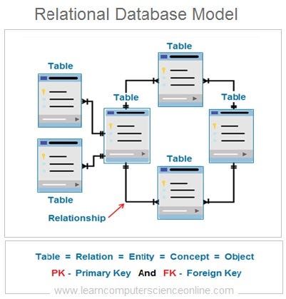
Relational Databases
In relational databases, the data is stored in tabular format grouped into rows and columns (similar to spreadsheets). A collection of rows is called a table. Each row represents a single record in the table and is made up of one or more columns.
These kinds of databases are relational because a relation is a mathematical idea equivalent to a table. So relational databases are databases that store their data in tables.
Tables
Below are some basic facts about tables:
Tables organize data in rows and columns.
Each row in a table represents one distinct record.
Each column represents a field or attribute that is common to all the records.
Fields should have a descriptive name and a data type appropriate for the attribute it represents.
Tables usually have more rows than columns.
Tables have primary keys that uniquely identify each row.
Foreign keys represent the relationships with other tables.
SQL is a standard language, which means that it almost certainly will be supported, no matter how your database is managed. That said, be aware that the SQL language can vary depending on database management tools. This lesson focuses on a set of core commands that never change. Learning the standard commands is an excellent introduction since the knowledge transfers between database products.
The syntax for SQL is English-like and requires fewer symbols than programming languages like C, Java, and JavaScript.
It is declarative and concise, which means there is a lot less to learn to use it effectively.
When learning SQL, it is helpful to understand that each command is designed for a different purpose. If we classify the commands by purpose, we'll end up with the following sub-categories of SQL:
- Data Definition Language (DDL): used to modify database objects. Some examples are:
CREATE TABLE,ALTER TABLE, andDROP TABLE. - Data Manipulation Language (DML): used to manipulate the data stored in the database. Some examples are:
INSERT,UPDATE, andDELETE. - Data Query Language (DQL): used to ask questions about the data stored in the database. The most commonly used SQL command is
SELECT, and it falls in this category. - Data Control Language (DCL): used to manage database security and user's access to data. These commands fall into the realm of Database Administrators. Some examples are
GRANTandREVOKE. - Transaction Control Commands: used for managing groups of statements that must execute as a unit or not execute at all. Examples are
COMMITandROLLBACK.
As a developer, you'll need to get familiar with DDL and become proficient using DML and DQL. This lesson will cover only DML and DQL commands.
Query
A query is a SQL statement used to retrieve data from a database. The command used to write queries is SELECT, and it is one of the most commonly used SQL commands.
The basic syntax for a SELECT statement is this:
select <selection> from <table name>;To see all the fields on a table, we can use a * as the selection.
select * from employees;The preceding statement would show all the records and all the columns for each record in the employees table.
To pick the fields we want to see, we use a comma-separated list:
select first_name, last_name, salary from employees;The return of that statement would hold all records from the listed fields.
We can extend the SELECT command's capabilities using clauses for things like filtering, sorting, pagination, and more.
It is possible to query multiple tables in a single query. But, in this section, we only perform queries on a single table. We will cover performing queries on multiple tables in another section.
Insert
To insert new data into a table, we'll use the INSERT command. The basic syntax for an INSERT statement is this:
insert into <table name> (<selection>) values (<values>)Using this formula, we can specify which values will be inserted into which fields like so:
insert into Customers (Country, CustomerName, ContactName, Address, City, PostalCode)
values ('USA', 'WebDev School', 'Austen Allred', '1 WebDev Court', 'Provo', '84601');
Modify
Modifying a database consists of updating and removing records. For these operations, we'll use UPDATE and DELETE commands, respectively.
The basic syntax for an UPDATE statement is:
update <table name> set <field> = <value> where <condition>;The basic syntax for a DELETE statement is:
delete from <table name> where <condition>;When querying a database, the default result will be every entry in the given table. However, often, we are looking for a specific record or a set of records that meets certain criteria.
A WHERE clause can help in both cases.
Here's an example where we might only want to find customers living in Berlin.
select City, CustomerName, ContactName
from Customers
where City = 'Berlin'
We can also chain together WHERE clauses using OR and AND to limit our results further.
The following query includes only records that match both criteria.
select City, CustomerName, ContactName
from Customers
where Country = 'France' and City = 'Paris'
And this query includes records that match either criteria.
select City, CustomerName, ContactName
from Customers
where Country = 'France' or City = 'Paris'
These operators can be combined and grouped with parentheses to add complex selection logic. They behave similarly to what you're used to in programming languages.
You can read more about SQLite operators from w3resource (Links to an external site.).
To select a single record, we can use a WHERE statement with a uniquely identifying field, like an id:
select * from Customers
where CustomerId=3;
Other comparison operators also work in WHERE conditions, such as >, <, <=, and >=.
select * from employees where salary >= 50000Ordering results using the ORDER BY clause
Query results are shown in the same order the data was inserted. To control how the data is sorted, we can use the ORDER BY clause. Let's see an example.
-- sorts the results first by salary in descending order, then by the last name in ascending order
select * from employees order by salary desc, last_name;
We can pass a list of field names to order by and optionally choose asc or desc for the sort direction. The default is asc, so it doesn't need to be specified.
Some SQL engines also support using field abbreviations when sorting.
select name, salary, department from employees order by 3, 2 desc;In this case, the results are sorted by the department in ascending order first and then by salary in descending order. The numbers refer to the fields' position in the selection portion of the query, so 1 would be name, 2 would be salary, and so on.
Note that the WHERE clause should come after the FROM clause. The ORDER BY clause always goes last.
select * from employees where salary > 50000 order by last_name;Limiting results using the LIMIT clause
When we wish to see only a limited number of records, we can use a LIMIT clause.
The following returns the first ten records in the products table:
select * from products
limit 10
LIMIT clauses are often used in conjunction with ORDER BY. The following shows us the five cheapest products:
select * from products
order by price desc
limit 5
Inserting data using INSERT
An insert statement adds a new record to the database. All non-null fields must be listed out in the same order as their values. Some fields, like ids and timestamps, may be auto-generated and do not need to be included in an INSERT statement.
-- we can add fields in any order; the values need to be in the same ordinal position
-- the id will be assigned automatically
  insert into Customers (Country, CustomerName, ContactName, Address, City, PostalCode)
  values ('USA', 'WebDev School', 'Austen Allred', '1 WebDev Court', 'Provo', '84601');
The values in an insert statement must not violate any restrictions and constraints that the database has in place, such as expected datatypes. We will learn more about constraints and schema design in a later section.
Modifying recording using UPDATE
When modifying a record, we identify a single record or a set of records to update using a WHERE clause. Then we can set the new value(s) in place.
update Customers
set City = 'Silicon Valley', Country = 'USA'
where CustomerName = 'WebDev School'
Technically the WHERE clause is not required, but leaving it off would result in every record within the table receiving the update.
Removing records using DELETE
When removing a record or set of records, we need only identify which record(s) to remove using a WHERE clause:
delete from Customers
where CustomerName = 'WebDev School`;
Once again, the WHERE clause is not required, but leaving it off would remove every record in the table, so it's essential.
For example, instead of a raw SQL SELECT:
SELECT * FROM users;We could use a query builder to write the same logic in JavaScript:
db.select('*').from('users');Query builders are lightweight and easy to get off the ground, whereas ORMs use an object-oriented model and provide more heavy lifting within their rigid structure.
We will use a query builder called knex.js (Links to an external site.).
To use Knex in a repository, we'll need to add two libraries:
npm install knex sqlite3knex is our query builder library, and sqlite3 allows us to interface with a sqlite database. We'll learn more about sqlite and other database management systems in the following module. For now, know that you need both libraries.
Next, we use Knex to set up a config file:
const knex = require('knex');

const config = {
  client: 'sqlite3',
  connection: {
    filename: './data/posts.db3',
  },
  useNullAsDefault: true,
};

module.exports = knex(config);
To use the query builder elsewhere in our code, we need to call knex and pass in a config object. We'll be discussing Knex configuration more in a future module. Still, we only need the client, connection, and useNullAsDefault keys as shown above. The filename should point towards the pre-existing database file, which can be recognized by the .db3 extension.
GOTCHA: The file path to the database should be with respect to the root of the repo, not the configuration file itself.
Once Knex is configured, we can import the above config file anywhere in our codebase to access the database.
const db = require('../data/db-config.js);The db object provides methods that allow us to begin building queries.
SELECT using Knex
In Knex, the equivalent of SELECT * FROM users is:
db.select('*').from('users');There's a simpler way to write the same command:
db('users');Using this, we could write a GET endpoint.
router.get('/api/users', (req, res) => {
  db('users')
  .then(users => {
    res.json(users);
  })
  .catch (err => {
    res.status(500).json({ message: 'Failed to get users' });
  });
});NOTE: All Knex queries return promises.
Knex also allows for a where clause. In Knex, we could write SELECT * FROM users WHERE id=1 as
db('users').where({ id: 1 });This method will resolve to an array containing a single entry like so: [{ id: 1, name: 'bill' }].
Using this, we might add a GET endpoint where a specific user:
server.get('api/users/:id', (req, res) => {
  const { id } = req.params;

db('users').where({ id })
  .then(users => {
    // we must check the length to find our if our user exists
    if (users.length) {
      res.json(users);
    } else {
      res.status(404).json({ message: 'Could not find user with given id.' })
   })
  .catch (err => {
    res.status(500).json({ message: 'Failed to get user' });
  });
});
INSERT using Knex
In Knex, the equivalent of INSERT INTO users (name, age) VALUES ('Eva', 32) is:
db('users').insert({ name: 'Eva', age: 32 });The insert method in Knex will resolve to an array containing the newly created id for that user like so: [3].
UPDATE using Knex
In knex, the equivalent of UPDATE users SET name='Ava', age=33 WHERE id=3; is:
db('users').where({ id: 3 })
.update({name: 'Ava', age: 33 });
Note that the where method comes before update, unlike in SQL.
Update will resolve to a count of rows updated.
DELETE using Knex
In Knex, the equivalent of DELETE FROM users WHERE age=33; is:
db('users').where({ age: 33}).del();Once again, the where must come before the del. This method will resolve to a count of records removed.
Here's a small project you can practice with.
SQLlite Studio is an application that allows us to create, open, view, and modify SQLite databases. To fully understand what SQLite Studio is and how it works, we must also understand the concept of the Database Management Systems (DBMS).
What is a DBMS?
To manage digital databases we use specialized software called DataBase Management Systems (DBMS). These systems typically run on servers and are managed by DataBase Administrators (DBAs).
In less technical terms, we need a type of software that will allow us to create, access, and generally manage our databases. In the world of relational databases, we specifically use Relational Database Mangement Systems (RDBMs). Some examples are Postgres, SQLite, MySQL, and Oracle.
Choosing a DBMS determines everything from how you set up your database, to where and how the data is stored, to what SQL commands you can use. Most systems share the core of the SQL language that you've already learned.
In other words, you can expect SELECT, UPDATE, INSERT, WHERE , and the like to be the same across all DBMSs, but the subtleties of the language may vary.
What is SQLite?
SQLite is the DBMS, as the name suggests, it is a more lightweight system and thus easier to get set up than some others.
SQLite allows us to store databases as single files. SQLite projects have a .db3 extension. That is the database.
SQLite is not a database (like relational, graph, or document are databases) but rather a database management system.
Opening an existing database in SQLite Studio
One useful visual interface we might use with a SQLite database is called SQLite Studio. Install SQLITE Studio here. (Links to an external site.)
Once installed, we can use SQLite Studio to open any .db3 file from a previous lesson. We may view the tables, view the data, and even make changes to the database.
For a more detailed look at SQLite Studio, follow along in the video above.
A well-designed database schema keeps the data well organized and can help ensure high-quality data.
Note that while schema design is usually left to Database Administrators (DBAs), understanding schema helps when designing APIs and database logic. And in a smaller team, this step may fall on the developer.
When designing a single table, we need to ask three things:
- What fields (or columns) are present?
- What type of data do we expect for each field?
- Are there other restrictions needed for each column?
Looking at the following schema diagram for an accounts table, we can the answer to each other those questions:
Table Fields
Choosing which fields to include in a table is relatively straight forward. What information needs to be tracked regarding this resource? In the real world, this is determined by the intended use of the product or app.
However, this is one requirement every table should satisfy: a primary key. A primary key is a way to identify each entry in the database uniquely. It is most often represented as a auto-incrementing integer called id or [tablename]Id.
Datatypes
Each field must also have a specified datatype. The datatype available depends on our DBMS. Some supported datatype in SQLite include:
- Null: Missing or unknown information.
- Integer: Whole numbers.
- Real: Any number, including decimals.
- Text: Character data.
- Blob: a large binary object that can be used to store miscellaneous data.
Any data inserted into the table must match the datatypes determined in schema design.
Constraints
Beyond datatypes, we may add additional constraints on each field. Some examples include:
- Not Null: The field cannot be left empty
- Unique: No two records can have the same value in this field
- Primary key: — Indicates this field is the primary key. Both the not null and unique constraints will be enforced.
- Default: — Sets a default value if none is provided.
As with data types, any data that does not satisfy the schema constraints will be rejected from the database.
Another critical component of schema design is to understand how different tables relate to each other. This will be covered in later lesson.
Knex provides a schema builder, which allows us to write code to design our database schema. However, beyond thinking about columns and constraints, we must also consider updates.
When a schema needs to be updated, a developer must feel confident that the changes go into effect everywhere. This means schema updates on the developer's local machine, on any testing or staging versions, on the production database, and then on any other developer's local machines. This is where migrations come into play.
A database migration describes changes made to the structure of a database. Migrations include things like adding new objects, adding new tables, and modifying existing objects or tables.
To use migrations (and to make Knex setup easier), we need to use knex cli. Install knex globally with npm install -g knex.
This allows you to use Knex commands within any repo that has knex as a local dependency. If you have any issues with this global install, you can use the npx knex command instead.
Initializing Knex
To start, add the knex and sqlite3 libraries to your repository.
npm install knex sqlite3
We've seen how to use manually create a config object to get started with Knex, but the best practice is to use the following command:
knex initOr, if Knex isn't globally installed:
npx knex initThis command will generate a file in your root folder called knexfile.js. It will be auto populated with three config objects, based on different environments. We can delete all except for the development object.
module.exports = {

development: {
    client: 'sqlite3',
    connection: {
      filename: './dev.sqlite3'
    }
  }

};
We'll need to update the location (or desired location) of the database as well as add the useNullAsDefault option. The latter option prevents crashes when working with sqlite3.
module.exports = {

development: {
    // our DBMS driver
    client: 'sqlite3',
    // the location of our db
    connection: {
      filename: './data/database_file.db3',
    },
    // necessary when using sqlite3
    useNullAsDefault: true
  }

};
Now, wherever we configure our database, we may use the following syntax instead of hardcoding in a config object.
const knex = require('knex');

const config = require('../knexfile.js');

// we must select the development object from our knexfile
const db = knex(config.development);

// export for use in codebase
module.exports = db;
Knex Migrations
Once our knexfile is set up, we can begin creating migrations. Though it's not required, we are going to add an addition option to the config object to specify a directory for the migration files.
development: {
    client: 'sqlite3',
    connection: {
      filename: './data/produce.db3',
    },
    useNullAsDefault: true,
    // generates migration files in a data/migrations/ folder
    migrations: {
      directory: './data/migrations'
    }
  }
We can generate a new migration with the following command:
knex migrate:make [migration-name]
If we needed to create an accounts table, we might run:
knex migrate:make create-accounts
Note that inside data/migrations/ a new file has appeared. Migrations have a timestamp in their filenames automatically. Wither you like this or not, do not edit migration names.
The migration file should have both an up and a down function. Within the up function, we write the ended database changes. Within the down function, we write the code to undo the up functions. This allows us to undo any changes made to the schema if necessary.
exports.up = function(knex, Promise) {
  // don't forget the return statement
  return knex.schema.createTable('accounts', tbl => {
    // creates a primary key called id
    tbl.increments();
    // creates a text field called name which is both required and unique
    tbl.text('name', 128).unique().notNullable();
    // creates a numeric field called budget which is required
    tbl.decimal('budget').notNullable();
  });
};

exports.down = function(knex, Promise) {
  // drops the entire table
  return knex.schema.dropTableIfExists('accounts');
};
References for these methods are found in the schema builder section of the Knex docs (Links to an external site.).
At this point, the table is not yet created. To run this (and any other) migrations, use the command:
knex migrate:latest
Note if the database does not exist, this command will auto-generate one. We can use SQLite Studio to confirm that the accounts table has been created.
Changes and Rollbacks
If later down the road, we realize you need to update your schema, you shouldn't edit the migration file. Instead, you will want to create a new migration with the command:
knex migrate:make accounts-schema-update
Once we've written our updates into this file we save and close with:
knex migrate:latest
If we migrate our database and then quickly realize something isn't right, we can edit the migration file. However, first, we need to rolllback (or undo) our last migration with:
knex migrate:rollback
Finally, we are free to rerun that file with knex migrate latest.
NOTE: A rollback should not be used to edit an old migration file once that file has accepted into a main branch. However, an entire team may use a rollback to return to a previous version of a database.
Overview
Often we want to pre-populate our database with sample data for testing. Seeds allow us to add and reset sample data easily.
Follow Along
The Knex command-line tool offers a way to seed our database; in other words, pre-populate our tables.
Similarly to migrations, we want to customize where our seed files are generated using our knexfile
development: {
    client: 'sqlite3',
    connection: {
      filename: './data/produce.db3',
    },
    useNullAsDefault: true,
    // generates migration files in a data/migrations/ folder
    migrations: {
      directory: './data/migrations'
    },
    seeds: {
      directory: './data/seeds'
    }
  }
To create a seed run: knex seed:make 001-seedName
Numbering is a good idea because Knex doesn't attach a timestamp to the name like migrate does. Adding numbers to the file name, we can control the order in which they run.
We want to create seeds for our accounts table:
knex seed:make 001-accounts
A file will appear in the designated seed folder.
exports.seed = function(knex, Promise) {
  // we want to remove all data before seeding
  // truncate will reset the primary key each time
  return knex('accounts').truncate()
    .then(function () {
      // add data into insert
      return knex('accounts').insert([
        { name: 'Stephenson', budget: 10000 },
        { name: 'Gordon & Gale', budget: 40400 },
      ]);
    });
};
Run the seed files by typing:
knex seed:run
You can now use SQLite Studio to confirm that the accounts table has two entries.
Foreign keys are a type of table field used for creating links between tables. Like primary keys, they are most often integers that identify (rather than store) data. However, whereas a primary key is used to id rows in a table, foreign keys are used to connect a record in one table to a record in a second table.
Consider the following farms and ranchers tables.
The farm_id in the ranchers table is an example of a foreign key. Each entry in the farm_id (foreign key) column corresponds to an id (primary key) in the farms table. This allows us to track which farm each rancher belongs to while keeping the tables normalized.
If we could only see the ranchers table, we would know that John, Jane, and Jen all work together and that Jim and Jay also work together. However, to know where any of them work, we would need to look at the farms table.
Now that we understand the basics of querying data from a single table, let's move on to selecting data from multiple tables using JOIN operations.
Overview
We can use a JOIN to combine query data from multiple tables using a single SELECT statement.
There are different types of joins; some are listed below:
- inner joins.
- outer joins.
- left joins.
- right joins.
- cross joins.
- non-equality joins.
- self joins.
Using joins requires that the two tables of interest contain at least one field with shared information. For example, if a departments table has an id field, and an employee table has a departmentid_ field, and the values that exist in the id column of the departments table live in the departmentid_ field of the employee table, we can use those fields to join both tables like so:
select * from employees
join departments on employees.department_id = departments.id
This query will return the data from both tables for every instance where the ON condition is true. If there are employees with no value for departmentid or where the value stored in the field does not correspond to an existing id in the departments table, then that record will NOT be returned. In a similar fashion, any records from the departments table that don't have an employee associated with them will also be omitted from the results. Basically, if the id* does not show as the value of department_id for an employee, it won't be able to join.
We can shorten the condition by giving the table names an alias. This is a common practice. Below is the same example using aliases, picking which fields to return and sorting the results:
select d.id, d.name, e.id, e.first_name, e.last_name, e.salary
from employees as e
join departments as d
  on e.department_id = d.id
order by d.name, e.last_name
Notice that we can take advantage of white space and indentation to make queries more readable.
There are several ways of writing joins, but the one shown here should work on all database management systems and avoid some pitfalls, so we recommend it.
The syntax for performing a similar join using Knex is as follows:
db('employees as e')
  .join('departments as d', 'e.department_id', 'd.id')
  .select('d.id', 'd.name', 'e.first_name', 'e.last_name', 'e.salary')
Follow Along
A good explanation of how the different types of joins can be seen in this article from w3resource.com (Links to an external site.).
What is SQL Joins?
An SQL JOIN clause combines rows from two or more tables. It creates a set of rows in a temporary table.
How to Join two tables in SQL?
A JOIN works on two or more tables if they have at least one common field and have a relationship between them.
JOIN keeps the base tables (structure and data) unchanged.
Join vs. Subquery
- JOINs are faster than a subquery and it is very rare that the opposite.
- In JOINs the RDBMS calculates an execution plan, that can predict, what data should be loaded and how much it will take to processed and as a result this process save some times, unlike the subquery there is no pre-process calculation and run all the queries and load all their data to do the processing.
- A JOIN is checked conditions first and then put it into table and displays; where as a subquery take separate temp table internally and checking condition.
- When joins are using, there should be connection between two or more than two tables and each table has a relation with other while subquery means query inside another query, has no need to relation, it works on columns and conditions.
SQL JOINS: EQUI JOIN and NON EQUI JOIN
The are two types of SQL JOINS — EQUI JOIN and NON EQUI JOIN
- SQL EQUI JOIN :
The SQL EQUI JOIN is a simple SQL join uses the equal sign(=) as the comparison operator for the condition. It has two types — SQL Outer join and SQL Inner join.
- SQL NON EQUI JOIN :
The SQL NON EQUI JOIN is a join uses comparison operator other than the equal sign like >, <, >=, <= with the condition.
SQL EQUI JOIN : INNER JOIN and OUTER JOIN
The SQL EQUI JOIN can be classified into two types — INNER JOIN and OUTER JOIN
- SQL INNER JOIN
This type of EQUI JOIN returns all rows from tables where the key record of one table is equal to the key records of another table.
- SQL OUTER JOIN
This type of EQUI JOIN returns all rows from one table and only those rows from the secondary table where the joined condition is satisfying i.e. the columns are equal in both tables.
In order to perform a JOIN query, the required information we need are:
a) The name of the tablesb) Name of the columns of two or more tables, based on which a condition will perform.
Syntax:
FROM table1
join_type table2
[ON (join_condition)]
Parameters:
Pictorial Presentation of SQL Joins:

Sample table: company
Sample table: foods
To join two tables 'company' and 'foods', the following SQL statement can be used :
SQL Code:
SELECT  company.company_id,company.company_name,
foods.item_id,foods.item_name
FROM company,foods;
Copy
Output:
COMPAN COMPANY_NAME              ITEM_ID  ITEM_NAME
------ ------------------------- -------- ---------------
18     Order All                 1        Chex Mix
18     Order All                 6        Cheez-It
18     Order All                 2        BN Biscuit
18     Order All                 3        Mighty Munch
18     Order All                 4        Pot Rice
18     Order All                 5        Jaffa Cakes
18     Order All                 7        Salt n Shake
15     Jack Hill Ltd             1        Chex Mix
15     Jack Hill Ltd             6        Cheez-It
15     Jack Hill Ltd             2        BN Biscuit
15     Jack Hill Ltd             3        Mighty Munch
15     Jack Hill Ltd             4        Pot Rice
15     Jack Hill Ltd             5        Jaffa Cakes
15     Jack Hill Ltd             7        Salt n Shake
16     Akas Foods                1        Chex Mix
16     Akas Foods                6        Cheez-It
16     Akas Foods                2        BN Biscuit
16     Akas Foods                3        Mighty Munch
16     Akas Foods                4        Pot Rice
16     Akas Foods                5        Jaffa Cakes
16     Akas Foods                7        Salt n Shake
.........
.........
.........
Overview
While we can write database code directly into our endpoints, best practices dictate that all database logic exists in separate, modular methods. These files containing database access helpers are often called models
Follow Along
To handle CRUD operations for a single resource, we would want to create a model (or database access file) containing the following methods:
function find() {
}

function findById(id) {
}

function add(user) {
}

function update(changes, id) {
}

function remove(id) {
}
Each of these functions would use Knex logic to perform the necessary database operation.
function find() {
  return db('users');
}
For each method, we can choose what value to return. For example, we may prefer findById() to return a single user object rather than an array.
function findById(id) {
// first() returns the first entry in the db matching the query
  return db('users').where({ id }).first();
}
We can also use existing methods like findById() to help add() return the new user (instead of just the id).
function add(user) {
  db('users').insert(user)
    .then(ids => {
      return findById(ids[0]);
    });
}
Once all methods are written as desired, we can export them like so:
module.exports = {
  find,
  findById,
  add,
  update,
  delete,
}
…and use the helpers in our endpoints
const User = require('./user-model.js');

router.get('/', (req, res) => {
  User.find()
    .then(users => {
      res.json(users);
    })
    .catch( err => {});
});
There should no be knex code in the endpoints themselves.
Normalization is the process of designing or refactoring database tables for maximum consistency and minimum redundancy.
With objects, we're used to denormalized data, stored with ease of use and speed in mind. Non-normalized tables are considered ineffective in relational databases.
Data normalization is a deep topic in database design. To begin thinking about it, we'll explore a few basic guidelines and some data examples that violate these rules.
Normalization Guidelines
Each record has a primary key.
No fields are repeated.
All fields relate directly to the key data.
Each field entry contains a single data point.
There are no redundant entries.
Denormalized Data
This table has two issues. There is no proper id field (as multiple farms may have the same name), and multiple fields are representing the same type of data: animals.
While we have now eliminated the first two issues, we now have multiple entries in one field, separated by commas. This isn't good either, as its another example of denormalization. There is no "array" data type in a relational database, so each field must contain only one data point.
Now we've solved the multiple fields issue, but we created repeating data (the farm field), which is also an example of denormalization. As well, we can see that if we were tracking additional ranch information (such as annual revenue), that field is only vaguely related to the animal information.
When these issues begin arising in your schema design, it means that you should separate information into two or more tables.
Anomalies
Obeying the above guidelines prevent anomalies in your database when inserting, updating, or deleting. For example, imagine if the revenue of Beech Ranch changed. With our denormalized schema, it may get updated in some records but not others:
Similarly, if Beech Ranch shut down, there would be three (if not more) records that needed to be deleted to remove a single farm.
Thus a denormalized table opens the door for contradictory, confusing, and unusable data.
What issues does the following table have?
There are three types of relationships:
One to one.
One to many.
Many to many.
Determining how data is related can provide a set of guidelines for table representation and guides the use of foreign keys to connect said tables.
One to One Relationships
Imagine we are storing the financial projections for a series of farms.
We may wish to attach fields like farm name, address, description, projected revenue, and projected expenses. We could divide these fields into two categories: information related to the farm directly (name, address, description) and information related to the financial projections (revenue, expenses).
We would say that farms and projections have a one-to-one relationship. This is to say that every farm has exactly one projection, and every project corresponds to exactly one farm.
This data can be represented in two tables: farms and projections
The farm_id is the foreign key that links farms and projections together.
Notes about one-to-one relationships:
- The foreign key should always have a
uniqueconstraint to prevent duplicate entries. In the example above, we wouldn't want to allow multiple projections records for one farm. - The foreign key can be in either table. For example, we may have had a
projection_idin thefarmstable instead. A good rule of thumb is to put the foreign key in whichever table is more auxiliary to the other. - You can represent one-to-one data in a single table without creating anomalies. However, it is sometimes prudent to use two tables as shown above to keep separate concerns in separate tables.
One to Many Relationships
Now imagine, we are storing the full-time ranchers employed at each farm. In this case, each rancher would only work at one farm however, each farm may have multiple ranchers.
This is called a one-to-many relationship.
This is the most common type of relationship between entities. Some other examples:
- One
customercan have manyorders. - One
usercan have manyposts. - One
postcan have manycomments.
Manage this type of relationship by adding a foreign key on the "many" table of the relationship that points to the primary key on the "one" table. Consider the farms and ranchers tables.
In a many-to-many relationship, the foreign key (in this case farm_id) should not be unique.
Many to Many Relationships
If we want to track animals on a farm as well, we must explore the many-to-many relationship. A farm has multiple animals, and multiple of each type of animal is present at multiple different farms.
Some other examples:
- an
ordercan have manyproductsand the sameproductwill appear in manyorders. - a
bookcan have more than oneauthor, and anauthorcan write more than onebook.
To model this relationship, we need to introduce an intermediary table that holds foreign keys that reference the primary key on the related tables. We now have a farms, animals, and farm_animals table.
While each foreign key on the intermediary table is not unique, the combinations of keys should be unique.
We have to consider the way that delete and updates through our API will impact related data.
Foreign Key Setup
In Knex, foreign key restrictions don't automatically work. Whenever using foreign keys in your schema, add the following code to your knexfile. This will prevent users from entering bad data into a foreign key column.
development: {
  client: 'sqlite3',
  useNullAsDefault: true,
  connection: {
    filename: './data/database.db3',
  },
  // needed when using foreign keys
  pool: {
    afterCreate: (conn, done) => {
      // runs after a connection is made to the sqlite engine
      conn.run('PRAGMA foreign_keys = ON', done); // turn on FK enforcement
    },
  },
},
Migrations
Let's look at how we might track our farms and ranchers using Knex. In our migration file's up function, we would want to create two tables:
exports.up = function(knex, Promise) {
  return knex.schema
    .createTable('farms', tbl => {
      tbl.increments();
      tbl.string('farm_name', 128)
        .notNullable();
    })
    // we can chain together createTable
    .createTable('ranchers', tbl => {
      tbl.increments();
      tbl.string('rancher_name', 128);
      tbl.integer('farm_id')
        // forces integer to be positive
        .unsigned()
        .notNullable()
        .references('id')
        // this table must exist already
        .inTable('farms')
    })
};
Note that the foreign key can only be created after the reference table.
In the down function, the opposite is true. We always want to drop a table with a foreign key before dropping the table it references.
exports.down = function(knex, Promise) {
  // drop in the opposite order
  return knex.schema
    .dropTableIfExists('ranchers')
    .dropTableIfExists('farms')
};
In the case of a many-to-many relationship, the syntax for creating an intermediary table is identical, except for one additional piece. We need a way to make sure our combination of foreign keys is unique.
.createTable('farm_animals', tbl => {
  tbl.integer('farm_id')
    .unsigned()
    .notNullable()
    .references('id')
    // this table must exist already
    .inTable('farms')
  tbl.integer('animal_id')
    .unsigned()
    .notNullable()
    .references('id')
    // this table must exist already
    .inTable('animals')

// the combination of the two keys becomes our primary key
  // will enforce unique combinations of ids
  tbl.primary(['farm_id', 'animal_id']);
});
Seeds
Order is also a concern when seeding. We want to create seeds in the same order we created our tables. In other words, don't create a seed with a foreign key, until that reference record exists.
In our example, make sure to write the 01-farms seed file and then the 02-ranchers seed file.
However, we run into a problem with truncating our seeds, because we want to truncate 02-ranchers before 01-farms. A library called knex-cleaner provides an easy solution for us.
Run knex seed:make 00-cleanup and npm install knex-cleaner. Inside the cleanup seed, use the following code.
const cleaner = require('knex-cleaner');

exports.seed = function(knex) {
  return cleaner.clean(knex, {
    mode: 'truncate', // resets ids
    ignoreTables: ['knex_migrations', 'knex_migrations_lock'], // don't empty migration tables
  });
};
This removes all tables (excluding the two tables that track migrations) in the correct order before any seed files run.
Cascading
If a user attempt to delete a record that is referenced by another record (such as attempting to delete Morton Ranch when entries in our ranchers table reference that record), by default, the database will block the action. The same thing can happen when updating a record when a foreign key reference.
If we want that to override this default, we can delete or update with cascade. With cascade, deleting a record also deletes all referencing records, we can set that up in our schema.
.createTable('ranchers', tbl => {
    tbl.increments();
    tbl.string('rancher_name', 128);
    tbl.integer('farm_id')
    .unsigned()
    .notNullable()
    .references('id')
    .inTable('farms')
    .onUpdate('CASCADE');
    .onDelete('CASCADE')
})